Linear Algebra
1D Vector: A single value (a scalar).
2D Vector: A coordinate pair used to position a pixel on a screen.
Left Hand Side
The Left Hand Side () represents the transformation. It’s the combination of your variables () and your coefficients. In geometry, this side describes the “span” or the space you are working in [4.1].
Right Hand Side
The Right Hand Side () represents the target. It is a fixed vector or constant. To find a solution, the target vector must land somewhere within the space described by the LHS [4.1].
Linear Combination
Scalar Multiplication
and a scalar .
The scalar multiplication would be:
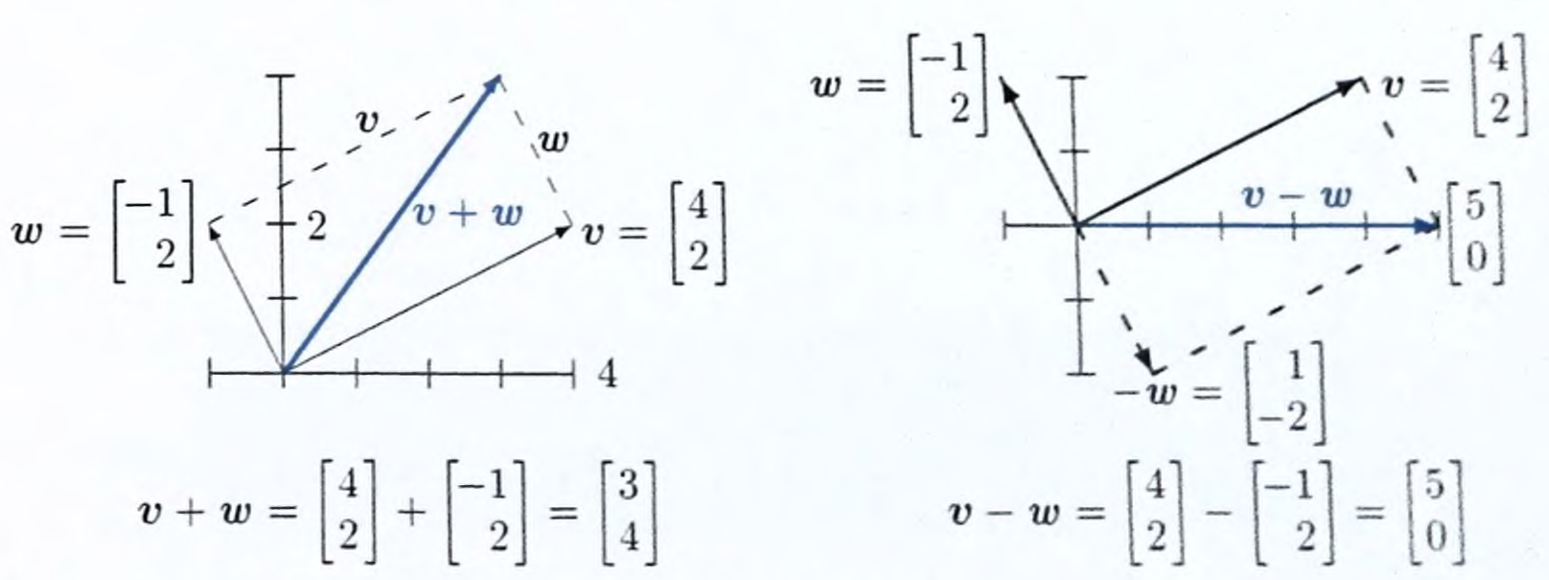
Vector Addition
and
The vector addition would be:
Dot Product
dot product is a single number that reveals the relationship between two vectors.
and
The number 11. It is no longer a point on a graph; it is a “score.”
This tells you how intense or strong the data is. example: In music: It’s the Volume. A loud song has a long vector; a quiet song has a short vector.
Schwarz Inequality
the length is
Length of is 5 (because ). The Length of is 2.23.
. (Maximum possible dot product you could get if two specific vectors were perfectly aligned)
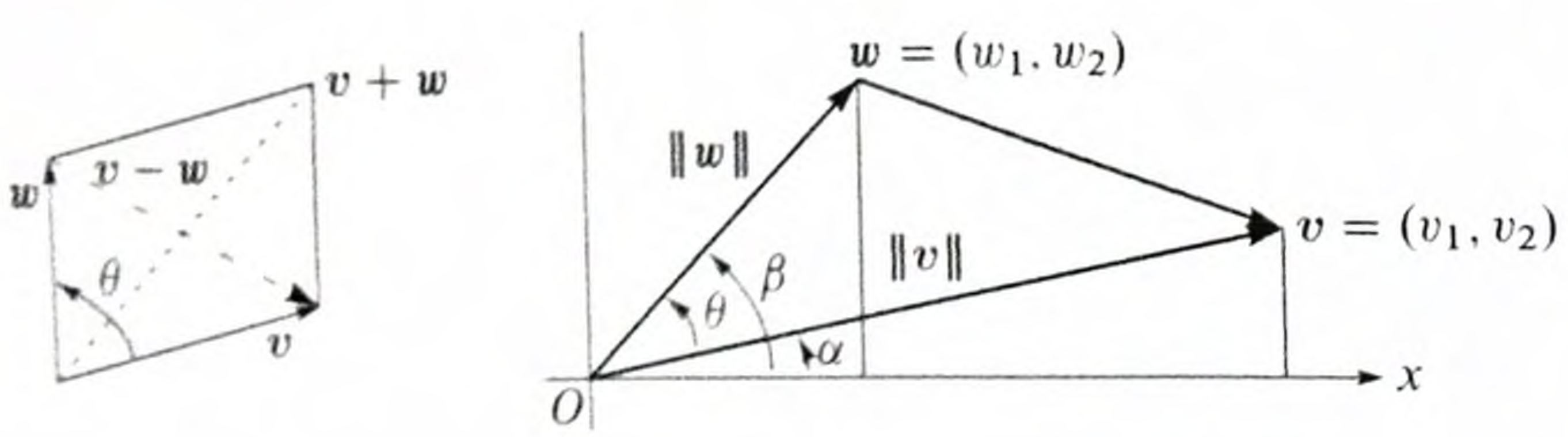
Cosine Rule (The Angle)
If a “Loud” song and a “Quiet” song are both Heavy Metal, they will point in the same direction (small angle).
- .
| If Similarity (Cosine) is… | The Angle (θ) is… | What it means |
|---|---|---|
| 1.00 | 0° | Perfectly identical direction. |
| 0.707 | 45° | Halfway between same and different. |
| 0.00 | 90° | Completely different (Perpendicular). |
Unit Vector
we often want to keep the direction of a vector but change its length to 1. This is called a Unit Vector ().
and its length is .
.
This “normalizes” data so you can compare different vectors fairly, regardless of how big the numbers started.
Triangle Inequality
It states that the shortest distance between two points is a straight line.
Example
- Home:
- Grocery Store: Point
- Coffee Shop: Point
First, you walk from Home to the Store, then from the Store to the Coffee Shop.
- Vector (Home to Store): You move 4 units East.
- Length
- Vector (Store to Coffee): You move 3 units North.
- Length
Total Distance of Path B:
If you had walked straight from Home to the Coffee Shop, you are looking for the length of the vector .
- Combined Vector:
- Length : Using Pythagoras:
Now we plug these numbers into the inequality:
The inequality is True. The straight line () is shorter than the two-step path ().
If you then walk from the Coffee Shop back to Home, you walk another units.
- Total Trip with the Store stop: units.
- Total Trip without the Store stop: units.
Matrix
If Matrix is and Matrix is , the resulting Matrix will be .
Top-Left Entry (Row 1 of A Column 1 of B)
Top-Right Entry (Row 1 of A Column 2 of B):
Bottom-Left Entry (Row 2 of A Column 1 of B):
Bottom-Right Entry (Row 2 of A Column 2 of B):
Linear Equations
linear equations in matrix form,
- Matrix (Coefficient Matrix): Contains only the numbers (coefficients) in front of the variables.
- Vector (Variable Vector): A column vector of the unknowns (e.g., ).
- Vector (Constant Vector): A column vector of the answers on the right side of the equals sign.
To write this in form:
Matrix Inner Product
is a way to take two matrices of the same size and produce a single scalar value. Any valid matrix inner product must satisfy four rules:
- Symmetry:
- Linearity:
- Additivity:
- Positivity: , and it only equals 0 if is a zero matrix.
The Frobenius Inner Product
For two real-valued matrices and of size , the inner product (denoted as ) is calculated by multiplying corresponding elements and summing them up.
There are three ways to write the same operation:
- Element-wise Sum:
- Using Trace:
- If you “flatten” both matrices into long vectors, their inner product is exactly the same as the standard vector dot product.
Just like the vector dot product tells us about the “relationship” between two arrows in space, the matrix inner product tells us about the relationship between two data structure:
-
Measuring Similarity: It tells us how “aligned” two matrices are. If the inner product is high, the matrices are similar; if it’s zero, the matrices are orthogonal.
-
Defining “Length” (Norm): The inner product of a matrix with itself gives the square of its “size,” known as the Frobenius Norm:
-
Projection: In machine learning and signal processing, we use inner products to “project” a data matrix onto a set of basis matrices (like in SVD or JPEG compression).
-
Optimization: Many loss functions in deep learning (like the cost of weights) are calculated using these types of inner products.
Suppose we have two matrices:
The inner product is:
Law Of Operations
| Operation | Law | Formula |
|---|---|---|
| Multiplication | Not Commutative | |
| Multiplication | Associative | |
| Transpose | Product Law | |
| Inverse | Product Law | |
| Scalar | Distributive |
Identity Matrix
Permutation Matrix
A permutation matrix of size has exactly one entry of 1 in each row and each column, with all other entries being 0.
For example, a permutation matrix might look like this:
Matrix Elimination
simplifying a complex fraction. make the matrix clean
Cost Of Elimination
| Phase | Operation Count (Approx) | Complexity |
|---|---|---|
| Forward Elimination | ||
| Back-Substitution | ||
| Total Solve Cost |
Augmented Matrix
Often, when solving these equations by hand (using a method like Gaussian Elimination), we use an Augmented Matrix.
To solve the equation we use
Gaussian Elimination
This method uses “row operations” to simplify the matrix into a form where we can read the answers.
We combine Matrix and Vector into one:
We want to eliminate the in the second row. We can do this by: Row 2 Row 2 Row 1).
New Matrix:
Back-Substitution
Now we turn the rows back into equations
- Bottom row:
- Top row:
- Substitute y:
Solution:
Matrix Inverse
inverse matrix is the mathematical “undo” button. Think of a matrix as a function that transforms data (moving a character in a game, encrypting a message, or blurring an image), the inverse is the function that reverses that transformation exactly.
()
When you multiply a matrix by its inverse, you get the Identity Matrix.
This method is like basic algebra. If , then . In matrices, we multiply by the inverse instead of dividing.
For a matrix , the inverse is .
Determinant:
Swap and Negate: Swap 1 and 4, make 2 and 3 negative
Multiply by 1/Det:
Solution:
Factorization
LU Decomposition ()
This is the matrix version of Gaussian Elimination. L stands for Lower Triangular, and U stands for Upper Triangular.
Identify the Pivot. The first pivot is (at position Row 1, Column 1).
Eliminate the value below the pivot.
We need to turn that into a . We do this by subtracting a multiple of Row 1 from Row 2.
- Multiplier (): .
- Operation:
The matrix is the “memory” of the elimination. Its job is to store the multipliers you used.
-
Start with the Identity: always starts as an Identity Matrix (1s on the diagonal, 0s elsewhere).
-
Insert the Multiplier: In Phase 1, we used the multiplier 4 to eliminate the value in Row 2, Column 1. We place that 4 in the exact same spot in .
Why is it 0 in the top right? Because we never use Row 2 to eliminate Row 1. We only work “downward,” so only the “lower” half of the matrix gets values
Instead of solving , which is slow, we solve two tiny, easy problems.
Imagine . We want to find in .
Step 1: Solve (Forward Substitution)
- Row 1:
- Row 2:
Step 2: Solve (Back Substitution)
- Row 2:
- Row 1:
Final Answer: .
QR Decomposition ()
This breaks a matrix into an Orthogonal matrix () and an Upper Triangular matrix (). Computers love orthogonal matrices because they don’t lose precision during calculations. This is the standard way to solve Least Squares problems (finding the best-fit line in Data Science).
-
Find : We use the Gram-Schmidt process to make the columns of orthonormal.
After normalizing, we get
-
Find : is calculated as .
Rank, Nullspace, and Columnspace
Nullspace
The Nullspace is the “Garbage Can” of a matrix. It consists of all the input vectors that the matrix “squashes” into zero.
If is in the nullspace, multiplying it by completely destroys its information, turning it into a vector of zeros
If the Nullspace is empty (only contains the zero vector): The matrix is “perfect.” Every unique input gives a unique output. You can reverse the process (Invert the matrix).
If the Nullspace has “stuff” in it: You have a problem. Multiple different inputs can produce the same output.
Matrix Rank
rank of a matrix is a single number that tells you how much “real” information is inside that matrix.
- Linearly Independent: This means a row is “unique.” You cannot create it by adding or scaling the other rows.
- Linearly Dependent: This means a row is a “copycat.” For example, if Row 2 is just Row 1 multiplied by 10, Row 2 is dependent and doesn’t count toward the rank.
Look at this matrix:
- Row 1:
- Row 2:
Notice that Row 2 is just Row 1. It adds no new information to the system. Because there is only one unique row, the Rank = 1.
Span, Subspace, Columnspace — A Unified Example
We will use 3D vectors where the numbers represent the amount of Cyan, Magenta, and Yellow ().
Row 1: Cyan Slot
Row 2: Yellow Slot
Row 3: Magenta Slot
The Span & Column Space
Col 1 (Cyan):
Col 2 (Yellow A):
Col 3 (Yellow B): (Oops! A duplicate of Col 2)
The Column Space is the Span of these three vectors. It represents every color this printer can make. Since we only have Cyan and Yellow ingredients, the span is “Every mix of Cyan and Yellow.”
The Vector Subspace (The “Result”)
Because we have no Magenta ingredient (the middle row of our result will always be 0 for the first and third components in a different setup, or specifically here, the third row is always 0), we are stuck in a 2D Subspace.
We can make (Green).
We can never make (Pure Magenta) because no combination of our columns can put a number in that bottom slot.
The Rank (The “Unique Info”)
Look at the columns again.
- Column 1 is unique.
- Column 2 is unique.
- Column 3 is just a copy of Column 2.
Since there are only 2 independent directions, the Rank = 2. Even though we have 3 cartridges, the printer only “sees” 2 dimensions of color.
The Nullspace (The “Waste”)
The Nullspace is the set of instructions that tells the printer to use ink, but results in zero color on the page ().
Since Column 2 and Column 3 are identical, watch what happens if we use this instruction:
This tells the printer: “Use 0 Cyan, 1 unit of Yellow A, and -1 unit of Yellow B.”
The ink cancels out! This vector is in the Nullspace. It represents a redundant command.
Singular Value Decomposition ()
SVD is a way of breaking down a complex table of data (a matrix) into its most basic, essential building blocks.
- (The “Who/What”): It identifies the categories or “latent features” in your data. (e.g., In a movie database, it might find categories like “Sci-Fi fans” or “Rom-Com fans”).
- (The “How Much”): It tells you the importance of each category. The first value is always the biggest “story” in your data; the last values are usually just random noise.
- (The “Connection”): It shows how the original items in your data relate to those new categories. (e.g., Which specific movies belong to the “Sci-Fi” category).
main purpose is to squint data, see hidden pattern, denoising